Vfrdtyky

Statistical mechanics
Thermodynamics Kinetic theory
Particle statistics Spin-statistics theorem Identical particles Maxwell–Boltzmann Bose–Einstein Fermi–Dirac Parastatistics Anyonic Statistics Braid Statistics
Thermodynamic ensembles NVE Microcanonical NVT Canonical µVT Grand canonical NPH Isoenthalpic–isobaric NPT Isothermal–isobaric
Models Debye Einstein Ising Potts
Potentials Internal energy Enthalpy Helmholtz free energy Gibbs free energy Grand potential / Landau free energy
Scientists Maxwell Boltzmann Gibbs Einstein Ehrenfest von Neumann Tolman Debye Fermi Bose
v t e

In quantum statistics, a branch of physics, Fermi–Dirac statistics describe a distribution of particles over energy states in systems consisting of many identical particles that obey the Pauli exclusion principle. It is named after Enrico Fermi and Paul Dirac, each of whom discovered the method independently (although Fermi defined the statistics earlier than Dirac).^[1][2]

Fermi–Dirac (F–D) statistics apply to identical particles with half-integer spin in a system with thermodynamic equilibrium. Additionally, the particles in this system are assumed to have negligible mutual interaction. That allows the many-particle system to be described in terms of single-particle energy states. The result is the F–D distribution of particles over these states which includes the condition that no two particles can occupy the same state; this has a considerable effect on the properties of the system. Since F–D statistics apply to particles with half-integer spin, these particles have come to be called fermions. It is most commonly applied to electrons, which are fermions with spin 1/2. Fermi–Dirac statistics are a part of the more general field of statistical mechanics and use the principles of quantum mechanics.

History

Before the introduction of Fermi–Dirac statistics in 1926, understanding some aspects of electron behavior were difficult due to seemingly contradictory phenomena. For example, the electronic heat capacity of a metal at room temperature seemed to come from 100 times fewer electrons than were in the electric current.^[3] It was also difficult to understand why those emission currents generated by applying high electric fields to metals at room temperature were almost independent of temperature.

The difficulty encountered by the electronic theory of metals at that time was due to considering that electrons were (according to classical statistics theory) all equivalent. In other words, it was believed that each electron contributed to the specific heat an amount on the order of the Boltzmann constant k_B.
This statistical problem remained unsolved until the discovery of F–D statistics.

F–D statistics was first published in 1926 by Enrico Fermi^[1] and Paul Dirac.^[2] According to Max Born, Pascual Jordan developed in 1925 the same statistics which he called Pauli statistics, but it was not published in a timely manner.^[4][5][6] According to Dirac, it was first studied by Fermi, and Dirac called it Fermi statistics and the corresponding particles fermions.^[7]

F–D statistics was applied in 1926 by R. Fowler to describe the collapse of a star to a white dwarf.^[8] In 1927 A. Sommerfeld applied it to electrons in metals^[9] and in 1928 Fowler and L.W. Nordheim applied it to field electron emission from metals.^[10] Fermi–Dirac statistics continues to be an important part of physics.

Fermi–Dirac distribution

For a system of identical fermions with thermodynamic equilibrium, the average number of fermions in a single-particle state i is given by a logistic function, or sigmoid function: the Fermi–Dirac (F–D) distribution,^[11]

n¯i=1e(ϵi−μ)/kBT+1{displaystyle {bar {n}}_{i}={frac {1}{e^{(epsilon _{i}-mu )/k_{rm {B}}T}+1}}}

where k_B is Boltzmann's constant, T is the absolute temperature, ε_i is the energy of the single-particle state i, and μ is the total chemical potential.

At zero temperature, μ is equal to the Fermi energy plus the potential energy per electron. For the case of electrons in a semiconductor, μ, the point of symmetry, is typically called the Fermi level or electrochemical potential.^[12][13]

The F–D distribution is only valid if the number of fermions in the system is large enough so that adding one more fermion to the system has negligible effect on μ.^[14] Since the F–D distribution was derived using the Pauli exclusion principle, which allows at most one electron to occupy each possible state, a result is that 0<n¯i<1{displaystyle 0<{bar {n}}_{i}<1} .^[15]

• Fermi–Dirac distribution


• 
  

  

  
  

  
  

  Energy dependence. More gradual at higher T. n¯{displaystyle {bar {n}}} = 0.5 when ϵ{displaystyle epsilon ;} = μ{displaystyle mu ;}. Not shown is that μ {displaystyle mu }decreases for higher T.^[16]

  
  

  
  


• 
  

  

  
  

  
  
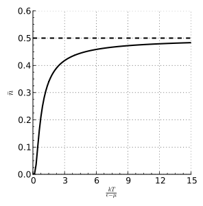
  Temperature dependence for ϵ>μ {displaystyle epsilon >mu } .
  

  
  

Distribution of particles over energy

Fermi function F(ϵ){displaystyle F(epsilon )} with μ = 0.55 eV for various temperatures in the range 50 K ≤ T ≤ 375 K

The above Fermi–Dirac distribution gives the distribution of identical fermions over single-particle energy states, where no more than one fermion can occupy a state. Using the F–D distribution, one can find the distribution of identical fermions over energy, where more than one fermion can have the same energy.^[17]

The average number of fermions with energy ϵi{displaystyle epsilon _{i}} can be found by multiplying the F–D distribution n¯i{displaystyle {bar {n}}_{i}} by the degeneracy gi{displaystyle g_{i}} (i.e. the number of states with energy ϵi{displaystyle epsilon _{i}}),^[18]

n¯(ϵi)=gin¯i=gie(ϵi−μ)/kBT+1.{displaystyle {begin{aligned}{bar {n}}(epsilon _{i})&=g_{i}{bar {n}}_{i}\&={frac {g_{i}}{e^{(epsilon _{i}-mu )/k_{rm {B}}T}+1}}.end{aligned}}}

When gi≥2{displaystyle g_{i}geq 2}, it is possible that n¯(ϵi)>1{displaystyle {bar {n}}(epsilon _{i})>1}, since there is more than one state that can be occupied by fermions with the same energy ϵi{displaystyle epsilon _{i}}.

When a quasi-continuum of energies ϵ{displaystyle epsilon } has an associated density of states g(ϵ){displaystyle g(epsilon )} (i.e. the number of states per unit energy range per unit volume^[19]), the average number of fermions per unit energy range per unit volume is

N¯(ϵ)=g(ϵ)F(ϵ),{displaystyle {bar {mathcal {N}}}(epsilon )=g(epsilon )F(epsilon ),}

where F(ϵ){displaystyle F(epsilon )} is called the Fermi function and is the same function that is used for the F–D distribution n¯i{displaystyle {bar {n}}_{i}},^[20]

F(ϵ)=1e(ϵ−μ)/kBT+1,{displaystyle F(epsilon )={frac {1}{e^{(epsilon -mu )/k_{rm {B}}T}+1}},}

so that

N¯(ϵ)=g(ϵ)e(ϵ−μ)/kBT+1.{displaystyle {bar {mathcal {N}}}(epsilon )={frac {g(epsilon )}{e^{(epsilon -mu )/k_{rm {B}}T}+1}}.}

Quantum and classical regimes

The classical regime, where Maxwell–Boltzmann statistics can be used as an approximation to Fermi–Dirac statistics, is found by considering the situation that is far from the limit imposed by the Heisenberg uncertainty principle for a particle's position and momentum. It can then be shown that the classical situation prevails when the concentration of particles corresponds to an average interparticle separation R¯{displaystyle {bar {R}}} that is much greater than the average de Broglie wavelength λ¯{displaystyle {bar {lambda }}} of the particles:^[21]

R¯≫λ¯≈h3mkBT,{displaystyle {bar {R}}gg {bar {lambda }}approx {frac {h}{sqrt {3mk_{rm {B}}T}}},}

where h is Planck's constant, and m is the mass of a particle.

For the case of conduction electrons in a typical metal at T = 300 K (i.e. approximately room temperature), the system is far from the classical regime because R¯≈λ¯/25{displaystyle {bar {R}}approx {bar {lambda }}/25} . This is due to the small mass of the electron and the high concentration (i.e. small R¯{displaystyle {bar {R}}}) of conduction electrons in the metal. Thus Fermi–Dirac statistics is needed for conduction electrons in a typical metal.^[21]

Another example of a system that is not in the classical regime is the system that consists of the electrons of a star that has collapsed to a white dwarf. Although the white dwarf's temperature is high (typically T = 7004100000000000000♠10000 K on its surface^[22]), its high electron concentration and the small mass of each electron precludes using a classical approximation, and again Fermi–Dirac statistics is required.^[8]

Derivations

Grand canonical ensemble

The Fermi–Dirac distribution, which applies only to a quantum system of non-interacting fermions, is easily derived from the grand canonical ensemble.^[23] In this ensemble, the system is able to exchange energy and exchange particles with a reservoir (temperature T and chemical potential µ fixed by the reservoir).

Due to the non-interacting quality, each available single-particle level (with energy level ϵ) forms a separate thermodynamic system in contact with the reservoir.
In other words, each single-particle level is a separate, tiny grand canonical ensemble.
By the Pauli exclusion principle, there are only two possible microstates for the single-particle level: no particle (energy E = 0), or one particle (energy E = ϵ). The resulting partition function for that single-particle level therefore has just two terms:

Z=exp⁡(0(μ−ϵ)/kBT)+exp⁡(1(μ−ϵ)/kBT)=1+exp⁡((μ−ϵ)/kBT),{displaystyle {begin{aligned}{mathcal {Z}}&=exp {big (}0(mu -epsilon )/k_{rm {B}}T{big )}+exp {big (}1(mu -epsilon )/k_{rm {B}}T{big )}\&=1+exp {big (}(mu -epsilon )/k_{rm {B}}T{big )},end{aligned}}}

and the average particle number for that single-particle level substate is given by

⟨N⟩=kBT1Z(∂Z∂μ)V,T=1exp⁡((ϵ−μ)/kBT)+1.{displaystyle langle Nrangle =k_{rm {B}}T{frac {1}{mathcal {Z}}}left({frac {partial {mathcal {Z}}}{partial mu }}right)_{V,T}={frac {1}{exp {big (}(epsilon -mu )/k_{rm {B}}T{big )}+1}}.}

This result applies for each single-particle level, and thus gives the Fermi–Dirac distribution for the entire state of the system.^[23]

The variance in particle number (due to thermal fluctuations) may also be derived (the particle number has a simple Bernoulli distribution):

⟨(ΔN)2⟩=kBT(d⟨N⟩dμ)V,T=⟨N⟩(1−⟨N⟩).{displaystyle {big langle }(Delta N)^{2}{big rangle }=k_{rm {B}}Tleft({frac {dlangle Nrangle }{dmu }}right)_{V,T}=langle Nrangle {big (}1-langle Nrangle {big )}.}

This quantity is important in transport phenomena such as the Mott relations for electrical conductivity and thermoelectric coefficient for an electron gas,^[24] where the ability of an energy level to contribute to transport phenomena is proportional to ⟨(ΔN)2⟩{displaystyle {big langle }(Delta N)^{2}{big rangle }}.

Canonical ensemble

It is also possible to derive Fermi–Dirac statistics in the canonical ensemble. Consider a many-particle system composed of N identical fermions that have negligible mutual interaction and are in thermal equilibrium.^[14] Since there is negligible interaction between the fermions, the energy ER{displaystyle E_{R}} of a state R{displaystyle R} of the many-particle system can be expressed as a sum of single-particle energies,

ER=∑rnrϵr{displaystyle E_{R}=sum _{r}n_{r}epsilon _{r};}

where nr{displaystyle n_{r}} is called the occupancy number and is the number of particles in the single-particle state r{displaystyle r} with energy ϵr{displaystyle epsilon _{r};}. The summation is over all possible single-particle states r{displaystyle r}.

The probability that the many-particle system is in the state R{displaystyle R}, is given by the normalized canonical distribution,^[25]

PR=e−βER∑R′e−βER′{displaystyle P_{R}={frac {e^{-beta E_{R}}}{displaystyle sum _{R'}e^{-beta E_{R'}}}}}

where β=1/kBT{displaystyle beta =1/k_{rm {B}}T}, e^{−βER{displaystyle scriptstyle -beta E_{R}}} is called the Boltzmann factor, and the summation is over all possible states R′{displaystyle R'} of the many-particle system.   The average value for an occupancy number ni{displaystyle n_{i};} is^[25]

n¯i = ∑Rni PR{displaystyle {bar {n}}_{i} = sum _{R}n_{i} P_{R}}

Note that the state R{displaystyle R} of the many-particle system can be specified by the particle occupancy of the single-particle states, i.e. by specifying n1,n2,…,{displaystyle n_{1},,n_{2},,ldots ;,} so that

PR=Pn1,n2,…=e−β(n1ϵ1+n2ϵ2+⋯)∑n1′,n2′,…e−β(n1′ϵ1+n2′ϵ2+⋯){displaystyle P_{R}=P_{n_{1},n_{2},ldots }={frac {e^{-beta (n_{1}epsilon _{1}+n_{2}epsilon _{2}+cdots )}}{displaystyle sum _{{n_{1}}',{n_{2}}',ldots }e^{-beta ({n_{1}}'epsilon _{1}+{n_{2}}'epsilon _{2}+cdots )}}}}

and the equation for n¯i{displaystyle {bar {n}}_{i}} becomes

n¯i=∑n1,n2,…ni Pn1,n2,…=∑n1,n2,…ni e−β(n1ϵ1+n2ϵ2+⋯+niϵi+⋯)∑n1,n2,…e−β(n1ϵ1+n2ϵ2+⋯+niϵi+⋯){displaystyle {begin{alignedat}{2}{bar {n}}_{i}&=sum _{n_{1},n_{2},dots }n_{i} P_{n_{1},n_{2},dots }\\&={frac {displaystyle sum _{n_{1},n_{2},dots }n_{i} e^{-beta (n_{1}epsilon _{1}+n_{2}epsilon _{2}+cdots +n_{i}epsilon _{i}+cdots )}}{displaystyle sum _{n_{1},n_{2},dots }e^{-beta (n_{1}epsilon _{1}+n_{2}epsilon _{2}+cdots +n_{i}epsilon _{i}+cdots )}}}\end{alignedat}}}

where the summation is over all combinations of values of n1,n2,…{displaystyle n_{1},n_{2},ldots ;}  which obey the Pauli exclusion principle, and nr{displaystyle n_{r}} = 0 or 1 for each r{displaystyle r}. Furthermore, each combination of values of n1,n2,…{displaystyle n_{1},n_{2},ldots ;} satisfies the constraint that the total number of particles is N{displaystyle N},

∑rnr=N.{displaystyle sum _{r}n_{r}=N.;}

Rearranging the summations,

n¯i=∑ni=01ni e−β(niϵi)∑∑(i)n1,n2,…⁡e−β(n1ϵ1+n2ϵ2+⋯)∑ni=01e−β(niϵi)∑∑(i)n1,n2,…⁡e−β(n1ϵ1+n2ϵ2+⋯){displaystyle {bar {n}}_{i}={frac {displaystyle sum _{n_{i}=0}^{1}n_{i} e^{-beta (n_{i}epsilon _{i})}quad sideset {}{^{(i)}}sum _{n_{1},n_{2},dots }e^{-beta (n_{1}epsilon _{1}+n_{2}epsilon _{2}+cdots )}}{displaystyle sum _{n_{i}=0}^{1}e^{-beta (n_{i}epsilon _{i})}qquad sideset {}{^{(i)}}sum _{n_{1},n_{2},dots }e^{-beta (n_{1}epsilon _{1}+n_{2}epsilon _{2}+cdots )}}}}

where the  (i){displaystyle ^{(i)}} on the summation sign indicates that the sum is not over ni{displaystyle n_{i}} and is subject to the constraint that the total number of particles associated with the summation is Ni=N−ni{displaystyle N_{i}=N-n_{i}} . Note that Σ(i){displaystyle Sigma ^{(i)}} still depends on ni{displaystyle n_{i}} through the Ni{displaystyle N_{i}} constraint, since in one case ni=0{displaystyle n_{i}=0} and Σ(i){displaystyle Sigma ^{(i)}} is evaluated with Ni=N,{displaystyle N_{i}=N,} while in the other case ni=1{displaystyle n_{i}=1} and Σ(i){displaystyle Sigma ^{(i)}} is evaluated with Ni=N−1.{displaystyle N_{i}=N-1.}  To simplify the notation and to clearly indicate that Σ(i){displaystyle Sigma ^{(i)}} still depends on ni{displaystyle n_{i}} through N−ni{displaystyle N-n_{i}} , define

Zi(N−ni)≡ ∑∑(i)n1,n2,…⁡e−β(n1ϵ1+n2ϵ2+⋯){displaystyle Z_{i}(N-n_{i})equiv sideset {}{^{(i)}}sum _{n_{1},n_{2},ldots }e^{-beta (n_{1}epsilon _{1}+n_{2}epsilon _{2}+cdots )};}

so that the previous expression for n¯i{displaystyle {bar {n}}_{i}} can be rewritten and evaluated in terms of the Zi{displaystyle Z_{i}},

n¯i =∑ni=01ni e−β(niϵi)  Zi(N−ni)∑ni=01e−β(niϵi)Zi(N−ni)= 0+e−βϵiZi(N−1)Zi(N)+e−βϵiZi(N−1)= 1[Zi(N)/Zi(N−1)]eβϵi+1.{displaystyle {begin{alignedat}{3}{bar {n}}_{i} &={frac {displaystyle sum _{n_{i}=0}^{1}n_{i} e^{-beta (n_{i}epsilon _{i})} Z_{i}(N-n_{i})}{displaystyle sum _{n_{i}=0}^{1}e^{-beta (n_{i}epsilon _{i})}qquad Z_{i}(N-n_{i})}}\\&= {frac {quad 0quad ;+e^{-beta epsilon _{i}};Z_{i}(N-1)}{Z_{i}(N)+e^{-beta epsilon _{i}};Z_{i}(N-1)}}\&= {frac {1}{[Z_{i}(N)/Z_{i}(N-1)];e^{beta epsilon _{i}}+1}}quad .end{alignedat}}}

The following approximation^[26] will be used to find an expression to substitute for Zi(N)/Zi(N−1){displaystyle Z_{i}(N)/Z_{i}(N-1)} .

ln⁡Zi(N−1)≃ln⁡Zi(N)−∂ln⁡Zi(N)∂N=ln⁡Zi(N)−αi{displaystyle {begin{alignedat}{2}ln Z_{i}(N-1)&simeq ln Z_{i}(N)-{frac {partial ln Z_{i}(N)}{partial N}}\&=ln Z_{i}(N)-alpha _{i};end{alignedat}}}

where      αi≡∂ln⁡Zi(N)∂N .{displaystyle alpha _{i}equiv {frac {partial ln Z_{i}(N)}{partial N}} .}

If the number of particles N{displaystyle N} is large enough so that the change in the chemical potential μ{displaystyle mu ;} is very small when a particle is added to the system, then αi≃−μ/kBT .{displaystyle alpha _{i}simeq -mu /k_{rm {B}}T .}^[27]  Taking the base e antilog^[28] of both sides, substituting for αi{displaystyle alpha _{i},}, and rearranging,

Zi(N)/Zi(N−1)=e−μ/kBT.{displaystyle Z_{i}(N)/Z_{i}(N-1)=e^{-mu /k_{rm {B}}T}.,}

Substituting the above into the equation for n¯i{displaystyle {bar {n}}_{i}}, and using a previous definition of β{displaystyle beta ;} to substitute 1/kBT{displaystyle 1/k_{rm {B}}T} for β{displaystyle beta ;}, results in the Fermi–Dirac distribution.

n¯i= 1e(ϵi−μ)/kBT+1{displaystyle {bar {n}}_{i}= {frac {1}{e^{(epsilon _{i}-mu )/k_{rm {B}}T}+1}}}

Like the Maxwell–Boltzmann distribution and the Bose–Einstein distribution the Fermi–Dirac distribution can also be derived by the Darwin–Fowler method of mean values (see Müller-Kirsten^[29]).

Microcanonical ensemble

A result can be achieved by directly analyzing the multiplicities of the system and using Lagrange multipliers.^[30]

Suppose we have a number of energy levels, labeled by index i, each level
having energy ε_i  and containing a total of n_i  particles. Suppose each level contains g_i  distinct sublevels, all of which have the same energy, and which are distinguishable. For example, two particles may have different momenta (i.e. their momenta may be along different directions), in which case they are distinguishable from each other, yet they can still have the same energy. The value of g_i  associated with level i is called the "degeneracy" of that energy level. The Pauli exclusion principle states that only one fermion can occupy any such sublevel.

The number of ways of distributing n_i indistinguishable particles among the g_isublevels of an energy level, with a maximum of one particle per sublevel, is given by the binomial coefficient, using its combinatorial interpretation

w(ni,gi)=gi!ni!(gi−ni)! .{displaystyle w(n_{i},g_{i})={frac {g_{i}!}{n_{i}!(g_{i}-n_{i})!}} .}

For example, distributing two particles in three sublevels will give population numbers of 110, 101, or 011 for a total of three ways which equals 3!/(2!1!).

The number of ways that a set of occupation numbers n_i can be realized is the product of the ways that each individual energy level can be populated:

W=∏iw(ni,gi)=∏igi!ni!(gi−ni)!.{displaystyle W=prod _{i}w(n_{i},g_{i})=prod _{i}{frac {g_{i}!}{n_{i}!(g_{i}-n_{i})!}}.}

Following the same procedure used in deriving the Maxwell–Boltzmann statistics,
we wish to find the set of n_i for which W is maximized, subject to the constraint that there be a fixed number of particles, and a fixed energy. We constrain our solution using Lagrange multipliers forming the function:

f(ni)=ln⁡(W)+α(N−∑ni)+β(E−∑niϵi).{displaystyle f(n_{i})=ln(W)+alpha (N-sum n_{i})+beta (E-sum n_{i}epsilon _{i}).}

Using Stirling's approximation for the factorials, taking the derivative with respect to n_i, setting the result to zero, and solving for n_i yields the Fermi–Dirac population numbers:

ni=gieα+βϵi+1.{displaystyle n_{i}={frac {g_{i}}{e^{alpha +beta epsilon _{i}}+1}}.}

By a process similar to that outlined in the Maxwell–Boltzmann statistics article, it can be shown thermodynamically that β=1kBT{textstyle beta ={frac {1}{k_{rm {B}}T}}} and α=−μkBT{textstyle alpha =-{frac {mu }{k_{rm {B}}T}}}, so that finally, the probability that a state will be occupied is:

n¯i=nigi=1e(ϵi−μ)/kBT+1.{displaystyle {bar {n}}_{i}={frac {n_{i}}{g_{i}}}={frac {1}{e^{(epsilon _{i}-mu )/k_{rm {B}}T}+1}}.}

Limiting behavior

The Fermi-Dirac distribution approaches the Maxwell-Boltzmann distribution in the limit of high temperature and low particle density, without the need for any ad hoc assumptions.

See also

Wikimedia Commons has media related to Fermi–Dirac distribution.

• Grand canonical ensemble


• Fermi level


• Maxwell–Boltzmann statistics


• Bose–Einstein statistics


• Parastatistics


• Logistic function

References

Further reading

• 
  Reif, F. (1965). Fundamentals of Statistical and Thermal Physics. McGraw–Hill. ISBN 978-0-07-051800-1.
  


• 
  Blakemore, J. S. (2002). Semiconductor Statistics. Dover. ISBN 978-0-486-49502-6.
  


• 
  Kittel, Charles (1971). Introduction to Solid State Physics (4th ed.). New York: John Wiley & Sons. ISBN 978-0-471-14286-7. OCLC 300039591.

References

^ ab Fermi, Enrico (1926). "Sulla quantizzazione del gas perfetto monoatomico". Rendiconti Lincei (in Italian). 3: 145–9..mw-parser-output cite.citation{font-style:inherit}.mw-parser-output q{quotes:"""""""'""'"}.mw-parser-output code.cs1-code{color:inherit;background:inherit;border:inherit;padding:inherit}.mw-parser-output .cs1-lock-free a{background:url("//upload.wikimedia.org/wikipedia/commons/thumb/6/65/Lock-green.svg/9px-Lock-green.svg.png")no-repeat;background-position:right .1em center}.mw-parser-output .cs1-lock-limited a,.mw-parser-output .cs1-lock-registration a{background:url("//upload.wikimedia.org/wikipedia/commons/thumb/d/d6/Lock-gray-alt-2.svg/9px-Lock-gray-alt-2.svg.png")no-repeat;background-position:right .1em center}.mw-parser-output .cs1-lock-subscription a{background:url("//upload.wikimedia.org/wikipedia/commons/thumb/a/aa/Lock-red-alt-2.svg/9px-Lock-red-alt-2.svg.png")no-repeat;background-position:right .1em center}.mw-parser-output .cs1-subscription,.mw-parser-output .cs1-registration{color:#555}.mw-parser-output .cs1-subscription span,.mw-parser-output .cs1-registration span{border-bottom:1px dotted;cursor:help}.mw-parser-output .cs1-hidden-error{display:none;font-size:100%}.mw-parser-output .cs1-visible-error{font-size:100%}.mw-parser-output .cs1-subscription,.mw-parser-output .cs1-registration,.mw-parser-output .cs1-format{font-size:95%}.mw-parser-output .cs1-kern-left,.mw-parser-output .cs1-kern-wl-left{padding-left:0.2em}.mw-parser-output .cs1-kern-right,.mw-parser-output .cs1-kern-wl-right{padding-right:0.2em}, translated as Zannoni, Alberto (1999-12-14). "On the Quantization of the Monoatomic Ideal Gas". arXiv:cond-mat/9912229.
^ ab Dirac, Paul A. M. (1926). "On the Theory of Quantum Mechanics". Proceedings of the Royal Society A. 112 (762): 661–77. Bibcode:1926RSPSA.112..661D. doi:10.1098/rspa.1926.0133. JSTOR 94692.
^ (Kittel 1971, pp. 249–50)
^ "History of Science: The Puzzle of the Bohr–Heisenberg Copenhagen Meeting". Science-Week. 4 (20). 2000-05-19. OCLC 43626035. Retrieved 2009-01-20.
^ Schücking: Jordan, Pauli, Politics, Brecht and a variable gravitational constant. In: Physics Today. Band 52, 1999, Heft 10
^ Ehlers, Schuecking: Aber Jordan war der Erste. In: Physik Journal. Band 1, 2002, Heft 11
^ Dirac, Paul A. M. (1967). Principles of Quantum Mechanics (revised 4th ed.). London: Oxford University Press. pp. 210–1. ISBN 978-0-19-852011-5.
^ ab Fowler, Ralph H. (December 1926). "On dense matter". Monthly Notices of the Royal Astronomical Society. 87 (2): 114–22. Bibcode:1926MNRAS..87..114F. doi:10.1093/mnras/87.2.114.
^ Sommerfeld, Arnold (1927-10-14). "Zur Elektronentheorie der Metalle" [On Electron Theory of Metals]. Naturwissenschaften (in German). 15 (41): 824–32. Bibcode:1927NW.....15..825S. doi:10.1007/BF01505083.
^ Fowler, Ralph H.; Nordheim, Lothar W. (1928-05-01). "Electron Emission in Intense Electric Fields" (PDF). Proceedings of the Royal Society A. 119 (781): 173–81. Bibcode:1928RSPSA.119..173F. doi:10.1098/rspa.1928.0091. JSTOR 95023.
^ (Reif 1965, p. 341)
^ (Blakemore 2002, p. 11)
^ Kittel, Charles; Kroemer, Herbert (1980). Thermal Physics (2nd ed.). San Francisco: W. H. Freeman. p. 357. ISBN 978-0-7167-1088-2.
^ ab (Reif 1965, pp. 340–2)
^ Note that n¯i{displaystyle {bar {n}}_{i}}is occupied, since no more than one fermion can occupy the same state at the same time and 0<n¯i<1{displaystyle 0<{bar {n}}_{i}<1}
^ (Kittel 1971, p. 245, Figs. 4 and 5)
^ These distributions over energies, rather than states, are sometimes called the Fermi–Dirac distribution too, but that terminology will not be used in this article.
^ Leighton, Robert B. (1959). Principles of Modern Physics. McGraw-Hill. p. 340. ISBN 978-0-07-037130-9.
Note that in Eq. (1), n(ϵ){displaystyle n(epsilon )}and ns{displaystyle n_{s}}
correspond respectively to n¯i{displaystyle {bar {n}}_{i}}
in this article. See also Eq. (32) on p. 339.
^ (Blakemore 2002, p. 8)
^ (Reif 1965, p. 389)
^ ab (Reif 1965, pp. 246–8)
^ Mukai, Koji; Jim Lochner (1997). "Ask an Astrophysicist". NASA's Imagine the Universe. NASA Goddard Space Flight Center. Archived from the original on 2009-01-20.
^ ab Srivastava, R. K.; Ashok, J. (2005). "Chapter 6". Statistical Mechanics. New Delhi: PHI Learning Pvt. Ltd. ISBN 9788120327825.
^ Cutler, M.; Mott, N. (1969). "Observation of Anderson Localization in an Electron Gas". Physical Review. 181 (3): 1336. Bibcode:1969PhRv..181.1336C. doi:10.1103/PhysRev.181.1336.
^ ab (Reif 1965, pp. 203–6)
^ See for example, Derivative - Definition via difference quotients, which gives the approximation f(a+h) ≈ f(a) + f '(a) h .
^ (Reif 1965, pp. 341–2) See Eq. 9.3.17 and Remark concerning the validity of the approximation.
^ By definition, the base e antilog of A is eA.
^ H.J.W. Müller-Kirsten, Basics of Statistical Physics, 2nd. ed., World Scientific (2013),
ISBN 978-981-4449-53-3.
^ (Blakemore 2002, pp. 343–5)